The final state of a black hole merger

Multipole Decomposition:

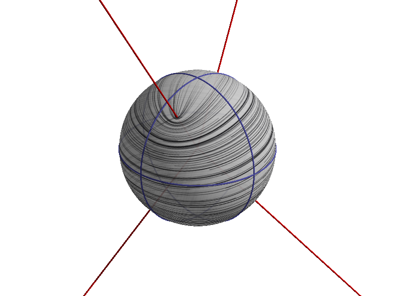
Stationary black holes have mass, spin, and charge. Astrophysical black holes are presumed to have negligible electric charge, so mass and spin are all that matter for astrophysics. But the black holes in numerical relativity simulations are not normally stationary. They begin in binary systems, where two black holes orbit around one another. As gravitational waves carry energy away from the system, and as other non-Newtonian effects begin to take over, the orbit decays until the holes come together and merge into one. This final black hole starts out with a highly distorted horizon, “peanut shaped” (with lobes corresponding to the progenitor horizons), which then settles down to a final stationary state. This final stationary state must be the so-called Kerr black hole, the stationary state with prescribed mass and spin.

This process of black hole “hair loss” was explored in great detail in the early 1970’s (a time now referred to as the “golden age of black hole research”), in which people applied techniques of black hole perturbation theory, where the deviations from stationarity are initially presumed to be “small”, and can then be shown to ring down to nothing.

The expectation was that similar behavior would occur in fully nonlinear general relativity. But until numerical codes were stable it was an impossible hypothesis to test. Even with numerical relativity, it’s a trickier project than you might guess. In textbooks, the Kerr black hole is defined by a particular “line element”, a formula defining the length of a path through spacetime. Unfortunately, this formula depends strongly on the choice of coordinates that label the points in space and time. The choice of coordinates is physically arbitrary and there’s no reason to presume that the coordinates that spacetime settles to at late times would correspond in any obvious way to any of the dozen or so coordinate systems that we use to describe Kerr black holes with pencil and paper. We have to look deeper than the mere mathematical formulas of the Kerr geometry. We need to coax out more fundamental geometrical structure, structure that we can compute without any reference to coordinates.

As it so happened, my work on black-hole spin just happened to provide such a structure. The spin angular momentum, aside from its relevance to spacetime symmetries, frame dragging, etc., is a particular component of a standard decomposition that we use in physics to describe the structure of objects. The multipole decomposition, in electromagnetism for example, breaks up a charge distribution into a monopole part (the overall charge), a dipole part (describing average displacement of positive from negative charges), and higher-order multipoles that describe further structure of the charge distribution. Along with this, there are current multipoles which describe the distribution of electrical current flow in electromagnetism.

In a beautiful paper, Ashtekar, Pawlowski, and Van Den Broeck argued that similar multipolar structure of black hole horizons could be described with a kind of spectral decomposition of quantities associated with the curvature of the horizon. By “spectral” decomposition, I mean that these curvature quantities are normally defined as functions of position on the horizon, but we can only describe “position” using coordinates, which are fundamentally arbitrary and best avoided. Instead, if we can find a set of functions, $y_\alpha$ , described by intrinsic horizon geometry, then we can define the multipole moments using integrals of curvature quantities against these functions. For example, the mass multipoles are described using integrals of the horizon scalar curvature $R$ : \begin{align} M_\alpha = \oint_{\cal H} y_\alpha R dA. \end{align}

In their work, Ashtekar et al. assumed the spacetime was symmetric around some axis, a condition that turns out to provide enough structure to define the functions $y_\alpha$ uniquely. Unfortunately in most binary black hole problems this structure disappears. Luckily, I’d just implemented in the SpEC code an alternative approach that happens to reduce the the approach of Ashtekar and collaborators in cases of axisymmetry. This alternative approach involves the eigenproblem that naturally arises in my treatment of black-hole spin: \begin{align} \nabla^4 y_\alpha + {\rm div}\left( R {\rm grad} (y_\alpha)\right) = \lambda_\alpha \nabla^2 y_\alpha, \end{align} where $\alpha$ is an index that labels all of the solutions to this eigenproblem.

Defining multipolar structure in this way turns out to automatically guarantee that the “current quadrupole moment” will coincide with the spin angular momentum, a fact that comfortably agrees with Newtonian results.

Defining multipolar structure in this way, I was able to show that the merger remnant in SpEC simulations settles down to Kerr geometry in an unambiguous sense. Along the way, the data showed an initial approximate symmetry (around the “peanut axis” of the initial merged hole) is quickly broken as the hole starts to ring down, and that a new symmetry (around the eventual spin axis) eventually arises. Most beautiful of all, each multipole quickly starts ringing down at precisely the frequencies and damping rates known from black-hole perturbation theory.

Algebraic Classification:

The multipolar structure of the horizon tells you about the horizon, which is certainly a very important part of a black hole. But there’s more to a black hole than just its horizon. A black hole is the tangle of spactime that’s left over after matter collapses, and to really have a complete picture of the structure of a black hole, you need to characterize not just the horizon, but also the spacetime around it.

Again, to do this, you can’t just hope to calculate the “gravitational field” and check whether it agrees with some standard formulas for the Kerr black hole, because the labelling of points in spacetime will generally be completely different in a numerical simulation than it is in the Kerr spacetime. You need to coax out more “basic”, more “invariant” characteristics of the spacetime geometry.

The purely-gravitational structure of spacetime geometry is encoded in a four-index field called the “Conformal Curvature Tensor”, or the “Weyl Tensor”: \begin{align} C_{\mu \nu \rho \sigma}. \end{align} I won’t give the (rather frightening) formula for this here. Suffice it to say that the Weyl tensor is a collection of quantities that vary from point to point in spacetime. It has four indices, and each one varies over the four coordinates of spacetime. So naively you’d think there would be $4^4 = 256$ of these components. However, the Weyl tensor satisfies a bunch of “index symmetries”, such as $C_{\nu \mu \rho \sigma} = - C_{\mu \nu \rho \sigma}$ , $C_{\mu \nu \sigma \rho} = - C_{\mu \nu \rho \sigma}$ , and $C_{\rho \sigma \mu \nu} = + C_{\mu \nu \rho \sigma}$ . These symmetries and others end up reducing the number of independent components of the Weyl tensor to ten. Still, these quantities are fundamentally dependent on how you label the points in spacetime, so you can’t just hope to compare them with known formulas to check whether a numerical spacetime settles down to the Kerr geometry.

One approach to coaxing out such information is called “algebraic classification” — find some special algebraic characteristic about the ten components of the Weyl tensor, a characteristic that’s independent of the labelling of points in spacetime, and use that to characterize the Weyl tensor. One such scheme of particular importance is called the Petrov classification. It can be described in a lot of different ways, but the most elegant way, I think, is due to Roger Penrose. Spacetime curvature has a lot of different consequences on the matter that moves through it, but the most immediate consequence is stretching and squeezing of the light rays that pass through the particular point under consideration. This stretching and squeezing, when it happens to light rays, is known as astigmatic focusing. This focusing depends not only on the point the light ray is passing through in space, but also on the direction that it’s propagating. For any Weyl tensor, it turns out that you can calculate four special directions along which light rays can pass without being squeezed by spacetime curvature. However, these special directions might be degenerate. That’s not a statement on their moral character, it’s just a way of saying that some of these four special directions might be the same. So this leads to a whole classification system. If all four of these special directions are different, the spacetime is said to be algebraically general, or Type I. If two of them are the same, but the other two are different, we say the spacetime is Type II. If three are the same and the fourth is different, Type III. If two are the same and the other two are different from the first but the same as each other, the spacetime is called Type D. If all four are the same, then the spacetime is Type N. The final case is when the Weyl tensor is zero, which ends up meaning there’s no focusing at all and hence no special dimensions, like the ordinary, boring, flat spacetime that we thought we lived in before Einstein came along. We call this Type O.

Petrov Classification These classifications are nested, in order of increasing specialization, as shown in this diagram. Each arrow points in a direction of increasing “specialness.” The classification scheme has a long and illustrious history in the study of exact (pencil-and-paper) solutions to Einstein’s field equations. In that context, one can begin with an ansatz about the algebraic type, and thereby reduce the full Einstein equations to a more tractable subset. Flat spacetime is type O. Plane gravitational wave spacetimes are generally type III or type N. The type of primary astrophysical interest is type D, because the black hole spacetimes of most interest there (Schwarzschild and Kerr) are everywhere type D. Rays propagating directly “away” from the hole, or directly “toward” it, are not lensed.

The point of computational general relativity is to study spacetimes with no symmetries and no special algebraic structure. The spacetimes that we study, such as the colliding black holes of gravitational-wave source simulations, are everywhere type I (algebraically general), however “near” the black holes, and long after they merge into a stationary remnant, they should become type D to a good approximation. Thus, checking that a numerical spacetime asymptotes to type D after the merger provides convincing and unambiguous evidence that it is settling down to the Kerr geometry. Moreover, it can be shown that the only stationary type D spacetimes (satisfying other easily-checked conditions) are Schwarzschild and Kerr. Thus, it not only provides compelling evidence, the approach to type D is a smoking gun.

Another group realized this fact and calculated relevant quantities in their numerical relativity simulations, to make just such an argument. They showed that indeed their simulations settle to type D at late times, and also that they mysteriously “hang up” in type II along the way. This apparent physical feature called out for a compelling physical explanation. I explored the question of how best to define “closeness” to a particular type of algebraic speciality, and in the process I showed that the apparent hangup in type II was not in fact a physical phenomenon, but rather an artifact of the mathematical tools used by the other group. I showed similar behavior in my own black-hole merger simulations, and then showed that it went away when I used better mathematical tools. Here is the paper in which I described these results.

These explorations provide two independent confirmations that when two black holes collide in general relativity, the remnant is another black hole, which exponentially settles to the Kerr geometry at late times. This outcome was widely expected, but not checked in any detail before this research. I was gratified that in a major review paper on the Kerr geometry, written for the centenary year of general relativity, this work was described as the most thorough analysis of the problem.

The multipole approach focuses on the structure of the horizon, and provides compelling physical language to describe not only that the spacetime settles to Kerr, but the process by which that occurs. I am planning further research, building on newer ideas from Ashtekar et al., to study the ringdown process in greater detail. I have also applied my Petrov Classification tools to other problems, most notably in collaboration with a student of mine who applied them the analysis of anisotropic cosmologies.